What happens when a transformer is allowed to redesign itself?
I started with two layers, a handful of structural operations, and a rule: changing the architecture must not destroy what the model already knows.
Most neural networks make their most consequential architectural decisions before seeing a single training example. Depth, width, and attention-head count are fixed in a configuration file, then optimization is asked to make the best of that shape. I wanted to test whether some of those decisions could move inside the training loop.
The result is a small language model whose plasticity controller inspects training signals every 500 steps. It can split, merge, or prune attention heads; duplicate or remove transformer layers; and expand the hidden dimension when the existing capacity appears saturated. The run described here trained on FineWeb-Edu for 30,000 steps on one A100.
The actual research question
The goal was not to make a tiny model competitive with large fixed transformers. At 6.9–10.4 million parameters, that would be the wrong comparison. The narrower question was whether gradient-derived signals could allocate capacity during training without producing a discontinuity in the model’s function.
That last clause is the difficult part. A controller that adds random layers can certainly make a network larger, but it also changes its output immediately and may invalidate the optimization state. Each operation therefore had to begin as close as possible to an identity transformation.
What the controller measures
Every 500 steps, the controller computes two families of signals. Head utility is the product of a head’s gradient norm and output norm. A head producing a large activation is not necessarily useful; the gradient term asks whether changing that output would affect the objective. Layer complexity is based on mean gradient magnitude and acts as a rough indication of how much pressure a layer is under.
These are deliberately simple heuristics. They are measurements that drive constrained decisions, not proof that the controller understands the network. Their value comes from being cheap enough to evaluate repeatedly and specific enough to map onto structural operations.
Six structural operations
- Split a head. A high-utility attention head is divided into two paths while preserving their combined contribution.
- Merge heads. Two heads that have learned sufficiently similar behavior are consolidated.
- Prune a head. A consistently low-utility head is removed rather than carried through the rest of training.
- Duplicate a layer. A high-complexity region receives additional depth.
- Remove a layer. Every dynamic layer has a learnable residual coefficient,
alpha. A layer whose coefficient falls to zero can disappear without changing the residual stream. - Grow the hidden dimension. Zero-padding utilities expand weights and optimizer-compatible tensors when the whole network appears saturated.
New layers enter with alpha = 0. At insertion they contribute nothing, so the model’s output is unchanged. Gradient descent must move that coefficient away from zero and make the new computation useful. If it fails, the controller can remove the layer again.
The 30,000-step run
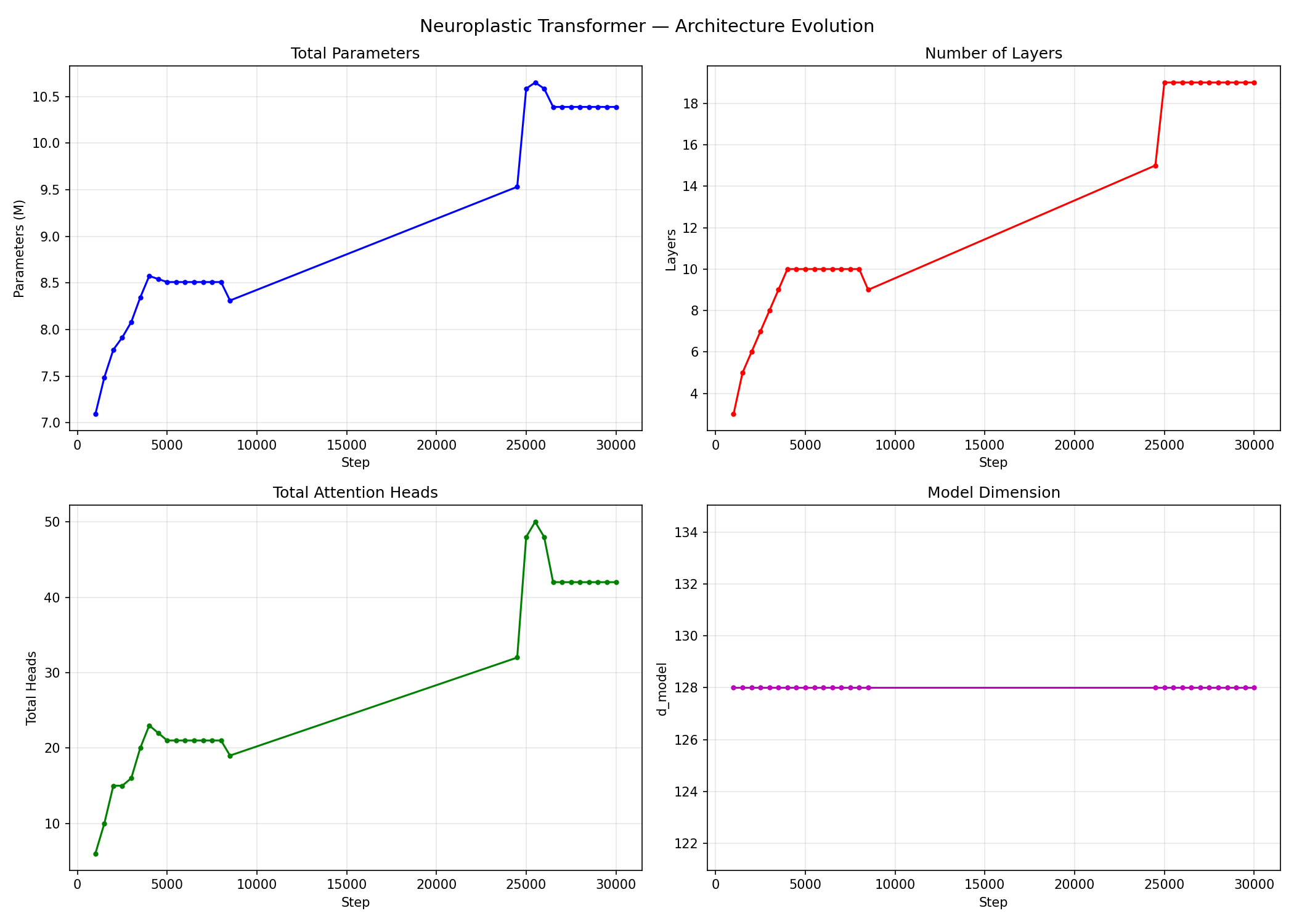
The model began with 2 layers, 4 total attention heads, a hidden size of 128, 6.9 million parameters, and a loss of 10.69. Training used a memory-mapped FineWeb-Edu token file when available, with a Hugging Face streaming path as fallback. The trainer supports single-GPU execution as well as torchrun/DDP, but this experiment used one A100 and took approximately 2 hours 16 minutes.
The controller made 236 structural changes. Growth was not monotonic. It repeatedly added depth, then removed layers that failed to develop useful residual weights. Between approximately steps 10,000 and 20,000, the network remained at 9 layers and made no architectural changes at all; it spent that interval refining weights. Around step 25,000, a second growth phase began and depth increased sharply.
The final network had 19 layers, 42 total attention heads, 10.4 million parameters, and a loss of 4.17. Hidden size remained 128. Layers 9–12 ended with three heads while the other layers stayed at two, producing a non-uniform allocation that was not specified in the initial configuration.
The event counts reveal a less tidy story than “the model grew.” There were 110 layer splits and 93 layer prunes, plus 14 head splits and 19 head merge/prune records. Eighty-one percent of all changes happened in the final 5,000 steps; at step 30,000 alone, the controller pruned eight layers and split eight layers in one invocation. That late churn may be useful exploration, or it may be a consequence of evaluating thresholds while the cosine learning rate is approaching zero.
The result I did not expect
Several layers learned negative alpha values. Layers 2, 9, 11, and 15 finished at approximately −0.16, −0.49, −0.04, and −0.53; layer 17 reached 1.50. In an ordinary residual block the transformation is added to the residual stream. A negative coefficient means the model learned to subtract that layer’s output instead. Alternating layers 4, 6, 8, 10, 12, 14, 16, and 18 remained near zero, suggesting that much of the late-added depth had not yet become consequential.
The experiment did not merely grow a deeper model. It produced a history of attempted capacity, rejected capacity, quiet periods, and a topology that became uneven.
Why this produced another tool
The trainer wrote snapshots, importance scores, metrics, and rewiring events. Those logs were enough to reproduce individual decisions but not enough to understand the complete trajectory. That observability problem became npviz: a separate recorder and dashboard for scrubbing through structural state, correlating rewiring with loss and gradient norm, and seeing where capacity moved over time.
What this run does not establish
This is one experimental run, not an independently reproduced result. The falling loss does not by itself show that adaptive growth outperforms a well-chosen fixed architecture. The controller also introduces thresholds and decision rules that are themselves hyperparameters. A fair evaluation needs fixed models matched by final parameter count and training compute, several random seeds, operation-by-operation ablations, controller-overhead measurements, and downstream evaluation beyond training loss.
Reproducing the path
The default entry point is python train.py; multi-GPU execution uses torchrun --nproc_per_node=4 train.py. FineWeb-Edu uses GPT-2 BPE (50,257 tokens), sequences of 512 tokens, and either a memory-mapped token file or Hugging Face streaming. The published run used FP16 autocast with gradient scaling, gradient clipping at 1.0, an effective batch of 65,536 tokens, AdamW, and a cosine schedule peaking at 6e-4 after 300 warm-up steps.
The Hugging Face release contains the paper, configuration, and a 111,820,451-byte step_30000.pt checkpoint. Its published configuration reports 19 layers and 10,387,219 parameters. I downloaded the checkpoint while preparing this page and verified SHA-256 555c640b…27c36; the interactive above intentionally reads the repository’s inspectable logs rather than making claims about tensors that require loading the checkpoint in PyTorch.
The next useful experiment is not “make it bigger.” It is to determine whether dynamic allocation buys anything measurable after accounting for its controller, its failed growth attempts, and the fixed baseline an informed practitioner would have chosen.
Read the source ↗Inspect the model ↗Read the paper (PDF) ↗Explore npviz ↗